US 2016 Election Analysis

Background Discussion

What makes predicting voter behavior (and thus election forecasting) a hard problem?

Many reasons may lead to the difficulty of predicting the voter behavior and election forecasting. The first one may be the number of voters for the 2016’s polls. While we expect that the equal number of Democrats and Republicians, it turned out that the Republican have much more voters than Democratic voters. Secondly, voters may change their decision. Several causes are whether or not the voter is a minority, their income earned, and the gender of those voters. We should analyze all those factors that may have influence on individual’s vote. What’s more, it turns out that many voters would change their vote in the week that leads up to voting according to previous elections. Last but not least, unpredictable future events that will happen. The society may change their attitude due to the news they’ve found on the TV or website, which is not predcitable.

Although Nate Silver predicted that Clinton would win 2016, he gave Trump higher odds than most. What is unique about Nate Silver’s methodology?

Compared to the usual approach which will take the maximum probabilty as the outcome, Nate Silver’s approach takes a full range of possibilities instead of just taking one maximum. For example, he calculated the possibilites of different dates of support and after calculation, he utilized the whole set of possibilities to model the shift in the polling numbers and thus get the desire result. He also looked at both the nation-level and test level votes. The whole idea of his approach is based on the Bayes’ Theorem.

Discuss why analysts believe predictions were less accurate in 2016. Can anything be done to make future predictions better? What are some challenges for predicting future elections? How do you think journalists communicate results of election forecasting models to a general audience

In the 2016, as we mentioned in the first question, the media plays a huge role for deciding which side of voters will be, the media overstated Clinton’s lead, especially in the Costal state. The news will lead to many voters choose Clintion, and feel uncomfortable with Trump. It is the same situation for the prediction of voting. So if we want to make the future prediction more precise, we might want to find out the potential news in the polictician. People should able to balance with the media’s instigate and their own thought. The challenges are clear because as people growing, their experience and knowledge is also growing, so next time maybe they will stick with their choice all the time instead of changing their decision last second. We think that journalists’ action may also lead to some violations to the model that we are trying to predict. It could cause some people to change their mind once again.

Data Wrangling

Remove summary rows in the election.raw data.

knitr::kable(election.raw %>% head) #take a look at the first cases
election = election.raw %>%
  filter(as.character(fips) != as.character(state) & fips !="US")

Finding the county level’s winner and state level’s winner

county_winner = election %>%
  group_by(fips) %>%
  mutate_at(vars(votes),funs(total=sum)) %>%
  mutate(pct = votes/total) %>%
  top_n(.,1,wt=pct)
state_winner = election %>%
  mutate(county=NULL, fips=NULL) %>%
  group_by(state) %>%
  mutate_at(vars(votes),funs(VotesInState=sum))%>%
  group_by(state,candidate) %>%
  mutate_at(vars(votes),funs(sum(votes)))%>%
  mutate(pct=votes/VotesInState)%>%
  group_by(state) %>%
  unique(.) %>%
  top_n(.,1,pct)

Visualization

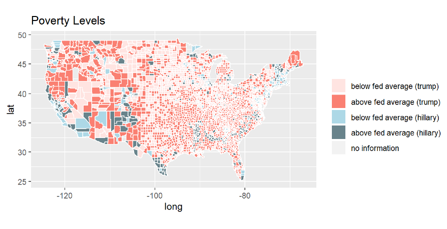
The following will show the map that visualizes the poverty level of each county, where the darker color of each group shows more federal poverty (above average) while the lighter color of each group represents less federal pvoerty(below average) in that region. For Trump we use the orange and blue for Hillary.As the result, we can see that Hillary has fewer ligiher color county with average lower rate of poverty compared to Trump.

Dimension Reduction

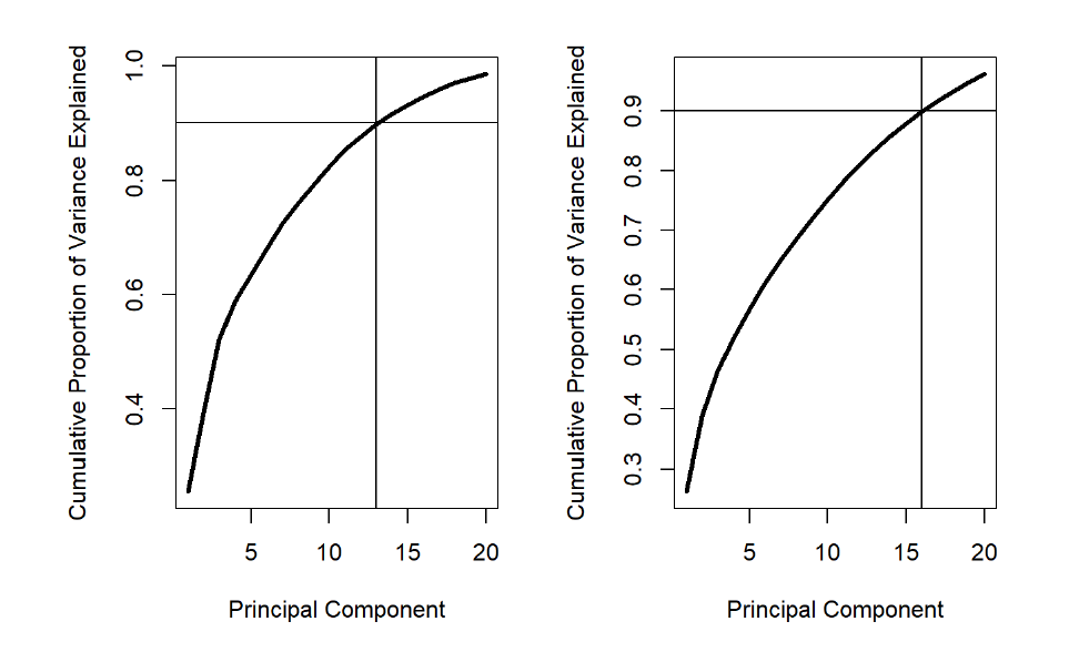
Using PCA for both county and sub-county data, both recentering and rescaling the dataset because the units is not the same for the dataset. Below is the plot that shows how many PCs explained 90% of the variance.

Classification

Decision Tree

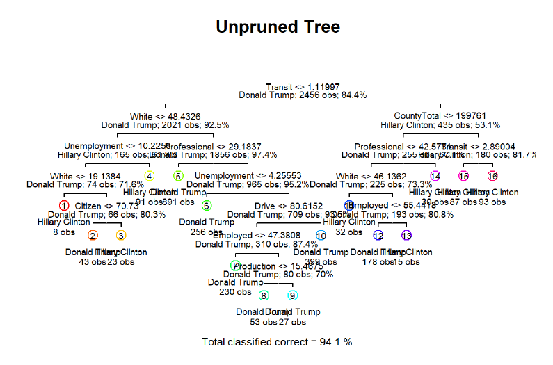
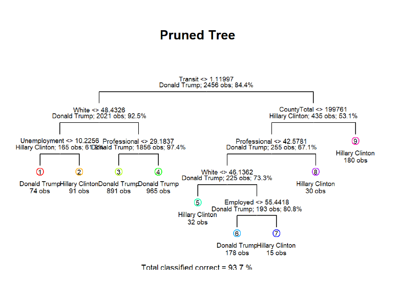
Pruning the tree to minimize the misclassfication error and prevent overfitting. As we can see above, the nodes reduced from 12 to 9.

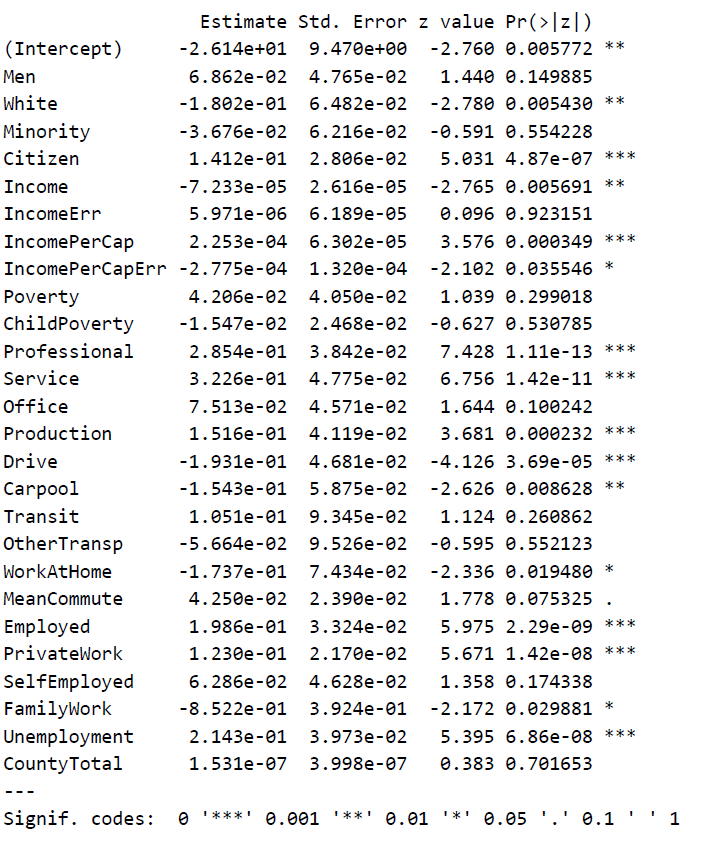
Logistic Regression

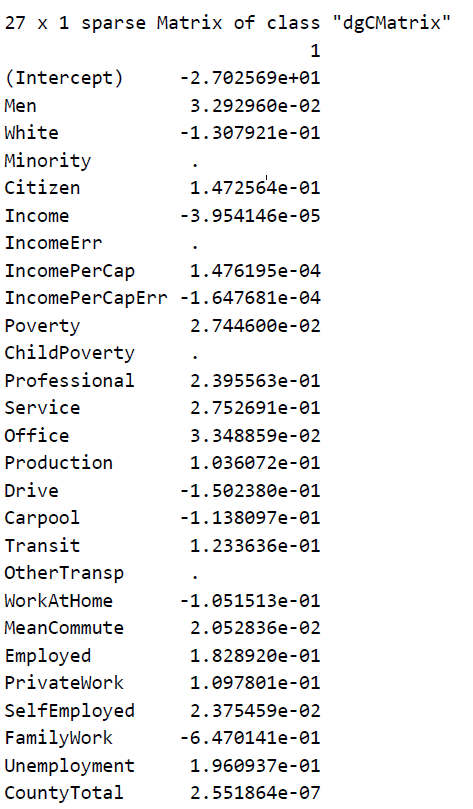
LASSO

ROC

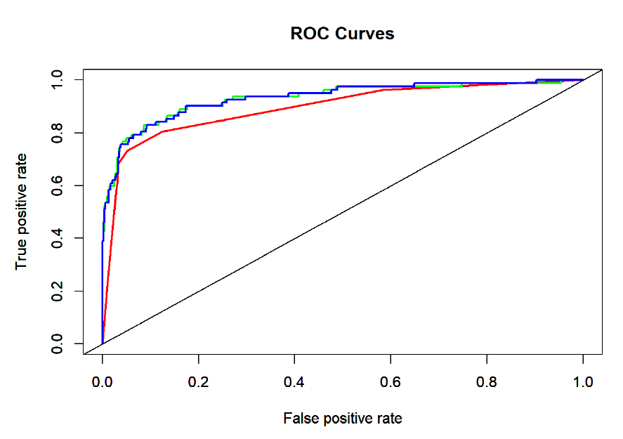Plotting the ROC curve, with red representing decision tree, green representing logistic regression, and blue representing LASSO.

Comparison

Method	train error	test error
Decision Tree	0.06270358	0.07003257
Logistic Regression	0.06921824	0.06514658
LASSO	0.06758958	0.06677524

Conclusion and Future Thoughts

This project shows that with so much difficuties to predict the election outcomes, we need to determine the most influential factors in order to form the most accurate predictions. We can see the raw data has some discrepancies like counties were split into 2 subcounties, some cities were classified as counties, and a few counties had missing data for the name variable. These kind of discrepancies make our job much more difficult to identify the voting outcomes for them.

We are declaring that we want to collecting addional data from past votings like the 2012 election to make the prediction more precise and analyze the data more clearly. We can figure out how many counties swithched their opinions from Democrates to Republicans for example. Also, when we get the data we can contrast the results from different times and locations to get more informations and try to simulate what will happen next.

Using KNN?

Method	train error	test error
Decision Tree	0.06270358	0.07003257
Logistic Regression	0.06921824	0.06514658
LASSO	0.06758958	0.06677524
KNN	0.1172638	0.1156352

We can see that the knn misclassification error is not low compared to the other methods we’ve used previously. Compared to the logistic regression and tree, we can see that logistic regression has the lowest error rate, which indicates that decision boundary for the candidates is probably on the linear side. Since KNN is non-parametric approach and with a linear boundry, we expect this kind of result from KNN classification. For the classfication trees, we can see the relationship between each variables is well approximated by a linear model then we will figure out that is not good compared to the logistic regression method. Our records error tells exactly what we are expecting to see. However, if we consider the difference between the two methods, it is not that significant, so we may still want to use decision tree because of its interpretability and visualization ability.

This simply shows outlines of the project, for more details please check this github repository